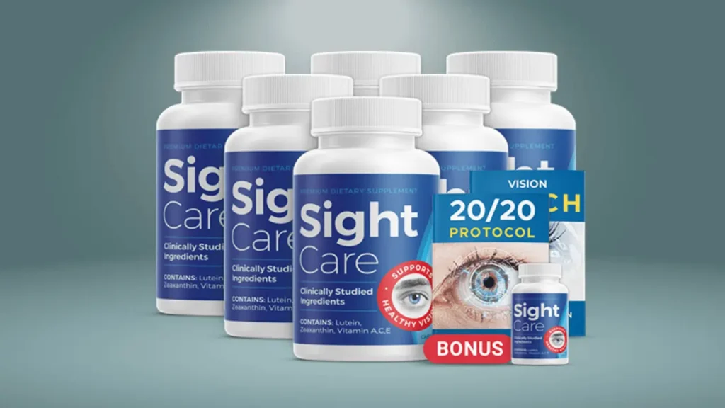
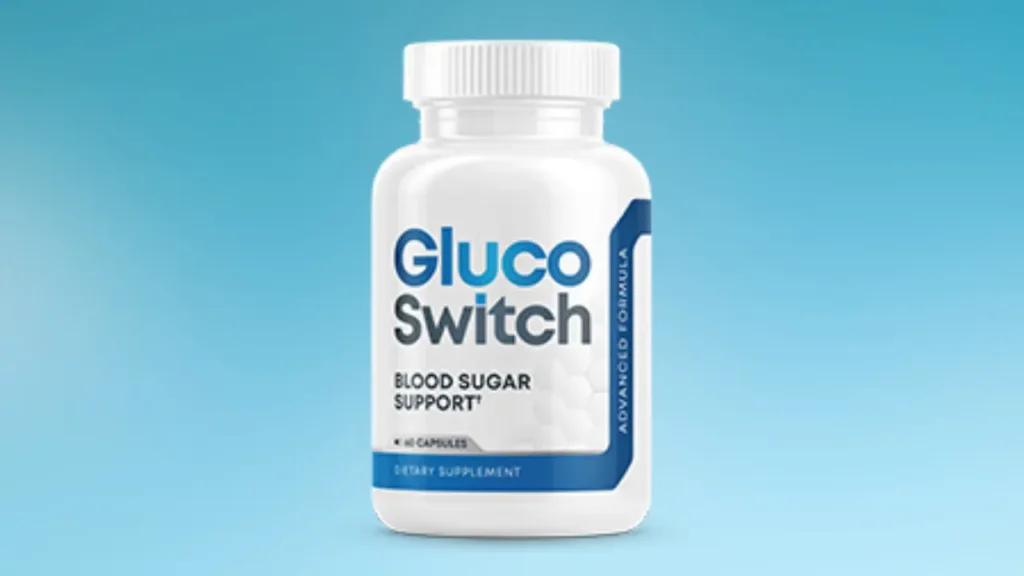
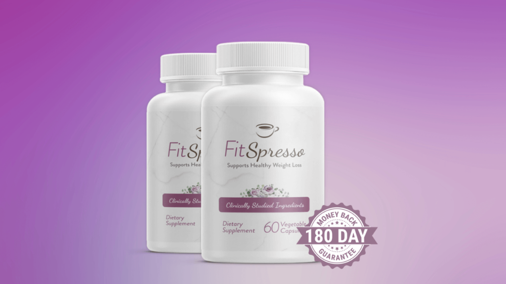
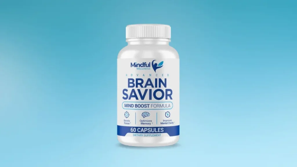
Imagine that you have a dataset with a list of predictors or independent variables and a list of targets or dependent variables. Then, by applying a decision tree like J48 on that dataset would allow you to predict the target variable of a new dataset record.
Decision tree J48 is the implementation of algorithm ID3 (Iterative Dichotomiser 3) developed by the WEKA project team. R includes this nice work into package RWeka. Let’s use it in the IRIS dataset. Flower specie will be our target variable, so we will predict it based on its measured features like Sepal or Petal length and width among others. # If not already, we should start by installing “RWeka” and “party” Packages
# Load both packages
# We will use dataset ‘IRIS’ from package ‘datasets’. It consists of 50 objects from each of three species of Iris flowers (Setosa, Virginica and Versicolor). For each object four attributes are measured length and width of sepal and petal.
# Using the decision tree ID3 in its J48 weka implementation, we want to predict the objective attribute “Species” based on attributes length and width of sepal and petal.
![]() How do we read this output ?Attribute Petal width is the one that contains much more information and for this reason it has been selected as the first split criteria. Reading the graphic we can notice that if Petal Width is less than 0.6 then there are 50 out of 150 objects that fall in Setosa. Otherwise if Petal Width is greater than 1.7 then there are 46 out of 150 objects that fall in Virginica … and so on. # To get the confusion matrix of J48 algorithm, type the following code.
We can see how J48 has taken a subset of IRIS as a training set and after that he has applied the resulting decision tree to the rest of IRIS dataset objects. Confusion Matrix is telling the following:
Open questions for students The decision tree has taken value 0.6 for Petal Width as split criteria. Why? |
How a decision tree works internallyBehind the idea of a decision tree we will find what it is called # The information gain calculation will answer the question of why the algorithm has decided to start with attribute Petal.Width.
The point is that attribute Petal.Width has information gain of 1.378, the highest in the IRIS dataset. # Let’s go further in this study. We will take a subset of IRIS which contains only objects with attribute Petal.Width > 0.6 and we will get the information gain of this subset.
Once again Petal.Width is the attribute which contains much more information and that is the reason why the second leave of the tree starts from the attribute Petal.Width. # Next step takes us to calculate the information gain of the subset which contains only objects with attribute Petal.Width <= 1.7
This time Petal.Length is the attribute with the highest information gain. In summary, Information gain is the mathematical tool that algorithm J48 has used to decide, in each tree node, which variable fits better in terms of target variable prediction. Pruning the decision treeWe will develop the importance of error tolerance parameter and the pruning concept in decision trees. __________ ) ) ) / (o o) < still working ! ooO–(_)–Ooo __________
You can also post any comment about this article, by visiting cRomoData.com |
J48 decision tree – Mining at UOC
Imagine that you have a dataset with a list of predictors or independent variables and a list of targets or dependent variables. Then, by applying a decision tree like J48 on that dataset would allow you to predict the target variable of a new dataset record. Decision tree J48 is […]